Training a Classifier

Open In Colab Download Jupyter Notebbok

Training a classifier on images is one of the most prominent examples showcasing what a library can do. Inspired by PyTorch’s tutorials, we want to train a convolutional neural network on the CIFAR10 dataset using the features of PyBlaze.

At first, we import all libraries that we’re going to use throughout this example:

import torch.nn as nn
import torch.nn.functional as F
import torch.optim as optim
import torchvision
import torchvision.transforms as transforms
import pyblaze.nn as xnn
import pyblaze.nn.functional as X
import matplotlib.pyplot as plt

%matplotlib inline

Loading the Data

At the beginning, we load our data conveniently using torchvision. PyBlaze does not come into play yet.

train_val_dataset = torchvision.datasets.CIFAR10(
    root="~/Downloads/", train=True, download=True, transform=transforms.Compose([
        transforms.RandomHorizontalFlip(),
        transforms.ToTensor()
    ])
)
test_dataset = torchvision.datasets.CIFAR10(
    root="~/Downloads/", train=False, download=True, transform=transforms.ToTensor()
)

Files already downloaded and verified
Files already downloaded and verified

Initializing Data Loaders

First, we set aside 20% of all training data for validation. Usually, you would need to compute the sizes of the resulting subsets and then split the dataset randomly. However, using PyBlaze, you can do this more conveniently.

By simply importing pyblaze.nn, datasets receive an additional function random_split. This accepts arbitrarily many floating point numbers indicating the fraction of the dataset to be randomly sampled into subsets. Note that these numbers need to add to 1.

train_dataset, val_dataset = train_val_dataset.random_split(0.8, 0.2)

Finally, we can initialize the data loaders. Normally, you would initialize a data loader and pass the dataset to the initializer. Again, as soon as you import pyblaze.nn, we extend PyTorch’s native dataset with a loader method. The method creates a data loader while its parameters are the same as for PyTorch’s data loader initializer.

train_loader = train_dataset.loader(batch_size=256, num_workers=4, shuffle=True)
val_loader = val_dataset.loader(batch_size=2048)
test_loader = test_dataset.loader(batch_size=2048)

Note that we set the batch size for validation and testing significantly higher than for training: as we are running the model in eval mode, no gradients need to be stored and much less memory is required.

Defining the Model

As a model, we define a common convolutional neural network. Most importantly, defining a model for PyBlaze is no different than defining a model natively in PyTorch. However, PyBlaze provides additional functionality to make it easier working with models.

A very useful layer that is introduced by PyBlaze is the xnn.View layer. While it is usually required to reshape the input in the forward method when using convolutional layers, xnn.View enables wrapping convolutional layers and linear layers into a single nn.Sequential module.

class Model(nn.Module):

    def __init__(self):
        super().__init__()

        self.seq = nn.Sequential(
            ConvNet(3, 32),
            ConvNet(32, 64),
            ConvNet(64, 128),
            xnn.View(-1, 2048),
            nn.Linear(2048, 10)
        )

    def forward(self, x):
        return self.seq(x)


class ConvNet(nn.Module):

    def __init__(self, in_channels, out_channels):
        super().__init__()

        self.conv = nn.Sequential(
            nn.Conv2d(in_channels, out_channels, 3, padding=1),
            nn.BatchNorm2d(out_channels),
            nn.ReLU(),
            nn.Conv2d(out_channels, out_channels, 3, padding=1),
            nn.BatchNorm2d(out_channels),
            nn.ReLU(),
            nn.MaxPool2d(2),
            nn.Dropout(0.25),
        )

    def forward(self, x):
        return self.conv(x)

Initializing a model is as simple as for pure PyTorch modules:

model = Model()

print(f"Model has {sum(p.numel() for p in model.parameters()):,} parameters.")

Model has 308,394 parameters.

Training the Model

Model training and evaluation is the core feature of PyBlaze. The code below trains the model according to the following constraints:

• We train with the data from train_loader and evaluate the performance after every epoch with data from val_loader.

• We train for 150 epochs (max), evaluate every 5 epochs and use early stopping with a patience of 5 evaluation steps. We simply use the default and track the validation loss.

• We use Adam with its default parameters as optimizer and minimize the cross entropy loss.

• We log the progress of each batch to the command line.

• We compute the accuracy of the predictions of the validation data after every epoch.

The result of this call is a history object which aggregates information about the training. This includes train losses after every batch as well as epoch. Further, it includes validation losses and validation metrics after every epoch.

engine = xnn.MLEEngine(model)
optimizer = optim.Adam(model.parameters(), lr=1e-3, weight_decay=1e-4)
loss = nn.CrossEntropyLoss()

history = engine.train(
    train_loader,
    val_data=val_loader,
    epochs=150,
    eval_every=5,
    optimizer=optimizer,
    loss=nn.CrossEntropyLoss(),
    callbacks=[
        xnn.BatchProgressLogger(),
        xnn.EarlyStopping(patience=5)
    ],
    metrics={
        'accuracy': X.accuracy
    }
)

Epoch 1/150:
 [Elapsed 0:00:04 | 34.36 it/s] loss: 1.45220, val_accuracy: 0.50680, val_loss: 1.48204
Epoch 2/150:
 [Elapsed 0:00:03 | 49.47 it/s] loss: 0.99612
Epoch 3/150:
 [Elapsed 0:00:03 | 50.81 it/s] loss: 0.83032
Epoch 4/150:
 [Elapsed 0:00:03 | 49.64 it/s] loss: 0.74560
Epoch 5/150:
 [Elapsed 0:00:03 | 51.70 it/s] loss: 0.68434
Epoch 6/150:
 [Elapsed 0:00:04 | 32.64 it/s] loss: 0.64454, val_accuracy: 0.77590, val_loss: 0.64798
Epoch 7/150:
 [Elapsed 0:00:03 | 49.65 it/s] loss: 0.60356
Epoch 8/150:
 [Elapsed 0:00:03 | 50.30 it/s] loss: 0.56721
Epoch 9/150:
 [Elapsed 0:00:03 | 51.20 it/s] loss: 0.54744
Epoch 10/150:
 [Elapsed 0:00:03 | 51.16 it/s] loss: 0.52634
Epoch 11/150:
 [Elapsed 0:00:04 | 34.72 it/s] loss: 0.50366, val_accuracy: 0.81740, val_loss: 0.53041
Epoch 12/150:
 [Elapsed 0:00:03 | 49.98 it/s] loss: 0.47945
Epoch 13/150:
 [Elapsed 0:00:03 | 50.96 it/s] loss: 0.46435
Epoch 14/150:
 [Elapsed 0:00:03 | 50.49 it/s] loss: 0.45264
Epoch 15/150:
 [Elapsed 0:00:03 | 49.38 it/s] loss: 0.43764
Epoch 16/150:
 [Elapsed 0:00:04 | 34.38 it/s] loss: 0.42418, val_accuracy: 0.83790, val_loss: 0.48021
Epoch 17/150:
 [Elapsed 0:00:03 | 50.63 it/s] loss: 0.41001
Epoch 18/150:
 [Elapsed 0:00:03 | 49.33 it/s] loss: 0.39783
Epoch 19/150:
 [Elapsed 0:00:03 | 50.42 it/s] loss: 0.38518
Epoch 20/150:
 [Elapsed 0:00:03 | 49.70 it/s] loss: 0.37354
Epoch 21/150:
 [Elapsed 0:00:04 | 34.07 it/s] loss: 0.36279, val_accuracy: 0.82470, val_loss: 0.51583
Epoch 22/150:
 [Elapsed 0:00:03 | 49.64 it/s] loss: 0.35568
Epoch 23/150:
 [Elapsed 0:00:02 | 52.38 it/s] loss: 0.34712
Epoch 24/150:
 [Elapsed 0:00:03 | 51.18 it/s] loss: 0.33781
Epoch 25/150:
 [Elapsed 0:00:03 | 51.23 it/s] loss: 0.33789
Epoch 26/150:
 [Elapsed 0:00:04 | 35.12 it/s] loss: 0.32599, val_accuracy: 0.85860, val_loss: 0.40353
Epoch 27/150:
 [Elapsed 0:00:03 | 51.04 it/s] loss: 0.31310
Epoch 28/150:
 [Elapsed 0:00:03 | 51.22 it/s] loss: 0.31169
Epoch 29/150:
 [Elapsed 0:00:03 | 50.33 it/s] loss: 0.30332
Epoch 30/150:
 [Elapsed 0:00:03 | 50.02 it/s] loss: 0.29768
Epoch 31/150:
 [Elapsed 0:00:04 | 32.99 it/s] loss: 0.29457, val_accuracy: 0.86270, val_loss: 0.40734
Epoch 32/150:
 [Elapsed 0:00:03 | 49.05 it/s] loss: 0.28917
Epoch 33/150:
 [Elapsed 0:00:03 | 48.90 it/s] loss: 0.28505
Epoch 34/150:
 [Elapsed 0:00:03 | 50.97 it/s] loss: 0.27621
Epoch 35/150:
 [Elapsed 0:00:03 | 51.19 it/s] loss: 0.26834
Epoch 36/150:
 [Elapsed 0:00:04 | 33.15 it/s] loss: 0.26322, val_accuracy: 0.85380, val_loss: 0.44287
Epoch 37/150:
 [Elapsed 0:00:03 | 51.53 it/s] loss: 0.25915
Epoch 38/150:
 [Elapsed 0:00:03 | 49.88 it/s] loss: 0.25473
Epoch 39/150:
 [Elapsed 0:00:03 | 50.75 it/s] loss: 0.26057
Epoch 40/150:
 [Elapsed 0:00:03 | 49.71 it/s] loss: 0.24920
Epoch 41/150:
 [Elapsed 0:00:04 | 32.96 it/s] loss: 0.24499, val_accuracy: 0.85930, val_loss: 0.43536
Epoch 42/150:
 [Elapsed 0:00:03 | 49.17 it/s] loss: 0.24057
Epoch 43/150:
 [Elapsed 0:00:03 | 50.87 it/s] loss: 0.23604
Epoch 44/150:
 [Elapsed 0:00:03 | 50.20 it/s] loss: 0.23447
Epoch 45/150:
 [Elapsed 0:00:03 | 50.96 it/s] loss: 0.23088
Epoch 46/150:
 [Elapsed 0:00:04 | 34.57 it/s] loss: 0.22833, val_accuracy: 0.86980, val_loss: 0.40272
Epoch 47/150:
 [Elapsed 0:00:03 | 50.16 it/s] loss: 0.22665
Epoch 48/150:
 [Elapsed 0:00:03 | 49.92 it/s] loss: 0.22133
Epoch 49/150:
 [Elapsed 0:00:03 | 50.30 it/s] loss: 0.22232
Epoch 50/150:
 [Elapsed 0:00:03 | 50.13 it/s] loss: 0.22184
Epoch 51/150:
 [Elapsed 0:00:04 | 34.80 it/s] loss: 0.21760, val_accuracy: 0.86400, val_loss: 0.42838
Epoch 52/150:
 [Elapsed 0:00:03 | 49.69 it/s] loss: 0.21549
Epoch 53/150:
 [Elapsed 0:00:03 | 50.43 it/s] loss: 0.21098
Epoch 54/150:
 [Elapsed 0:00:03 | 49.40 it/s] loss: 0.20790
Epoch 55/150:
 [Elapsed 0:00:03 | 50.09 it/s] loss: 0.20619
Epoch 56/150:
 [Elapsed 0:00:04 | 32.51 it/s] loss: 0.20051, val_accuracy: 0.87510, val_loss: 0.40508
Epoch 57/150:
 [Elapsed 0:00:03 | 49.84 it/s] loss: 0.19795
Epoch 58/150:
 [Elapsed 0:00:03 | 50.18 it/s] loss: 0.19924
Epoch 59/150:
 [Elapsed 0:00:03 | 50.01 it/s] loss: 0.19628
Epoch 60/150:
 [Elapsed 0:00:03 | 49.69 it/s] loss: 0.19570
Epoch 61/150:
 [Elapsed 0:00:04 | 33.88 it/s] loss: 0.19398, val_accuracy: 0.88240, val_loss: 0.38243
Epoch 62/150:
 [Elapsed 0:00:03 | 50.92 it/s] loss: 0.19323
Epoch 63/150:
 [Elapsed 0:00:03 | 49.32 it/s] loss: 0.19755
Epoch 64/150:
 [Elapsed 0:00:03 | 50.32 it/s] loss: 0.19354
Epoch 65/150:
 [Elapsed 0:00:03 | 51.20 it/s] loss: 0.18593
Epoch 66/150:
 [Elapsed 0:00:04 | 33.16 it/s] loss: 0.18705, val_accuracy: 0.86990, val_loss: 0.40923
Epoch 67/150:
 [Elapsed 0:00:03 | 50.13 it/s] loss: 0.17992
Epoch 68/150:
 [Elapsed 0:00:03 | 51.34 it/s] loss: 0.18269
Epoch 69/150:
 [Elapsed 0:00:03 | 49.79 it/s] loss: 0.18332
Epoch 70/150:
 [Elapsed 0:00:03 | 51.06 it/s] loss: 0.18073
Epoch 71/150:
 [Elapsed 0:00:04 | 34.35 it/s] loss: 0.18015, val_accuracy: 0.87790, val_loss: 0.39438
Epoch 72/150:
 [Elapsed 0:00:03 | 50.55 it/s] loss: 0.17447
Epoch 73/150:
 [Elapsed 0:00:03 | 50.53 it/s] loss: 0.17418
Epoch 74/150:
 [Elapsed 0:00:03 | 49.42 it/s] loss: 0.17548
Epoch 75/150:
 [Elapsed 0:00:03 | 50.86 it/s] loss: 0.17303
Epoch 76/150:
 [Elapsed 0:00:04 | 33.72 it/s] loss: 0.17062, val_accuracy: 0.85620, val_loss: 0.49162
Epoch 77/150:
 [Elapsed 0:00:03 | 49.73 it/s] loss: 0.17179
Epoch 78/150:
 [Elapsed 0:00:03 | 51.45 it/s] loss: 0.17274
Epoch 79/150:
 [Elapsed 0:00:03 | 50.71 it/s] loss: 0.17069
Epoch 80/150:
 [Elapsed 0:00:03 | 51.87 it/s] loss: 0.16697
Epoch 81/150:
 [Elapsed 0:00:04 | 33.46 it/s] loss: 0.16554, val_accuracy: 0.87900, val_loss: 0.40666
Epoch 82/150:
 [Elapsed 0:00:03 | 50.45 it/s] loss: 0.16777
Epoch 83/150:
 [Elapsed 0:00:03 | 49.40 it/s] loss: 0.16606
Epoch 84/150:
 [Elapsed 0:00:03 | 50.07 it/s] loss: 0.16360
Epoch 85/150:
 [Elapsed 0:00:03 | 50.44 it/s] loss: 0.16609
Epoch 86/150:
 [Elapsed 0:00:04 | 33.82 it/s] loss: 0.16356, val_accuracy: 0.86780, val_loss: 0.44691
Early stopping after epoch 86 (patience 5).

Plotting the Losses

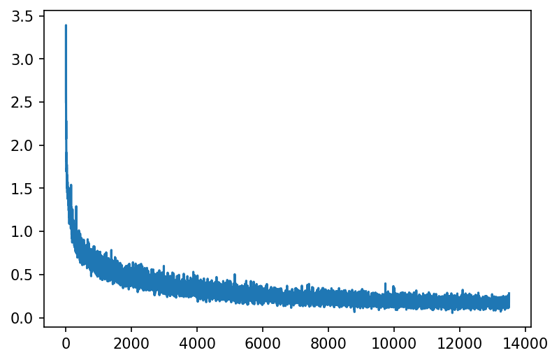
With the information from the history object, we can plot the progress of our training. The history object always provides batch_loss summarizing the training losses after each batch as well as loss as the train losses after each epoch. Depending on additional parameters passed to the fit function, additional keys are available.

all_losses = history.batch_loss
plt.figure(dpi=150)
plt.plot(range(len(all_losses)), all_losses)
plt.show()

In our case, we used validation and therefore there exists a val_loss property on the history object. Theoretically, we would also be able to plot val_accuracy as all metrics are recorded in the history object as well.

import numpy as np

plt.figure(dpi=150)
plt.plot(range(len(history.loss)), history.loss, label='Training Loss')
plt.plot(np.array(range(len(history.val_loss))) * 5, history.val_loss, label='Validation Loss')
plt.legend()
plt.show()

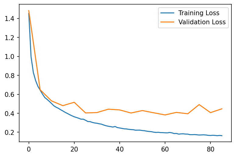
As we can see, the losses are starting to diverge and the generalization gap becomes larger starting from epoch 25. However, the lowest validation loss was obtained after epoch 61.

Evaluating the Model

Lastly, we want to evaluate the performance of our model. For this, we use our test data and call evaluate on the model. We are interested only in a single metric, the accuracy.

The returned value is a dictionary which provides the metrics that were recorded. In our case, the only metric is accuracy.

evaluation = engine.evaluate(
    test_loader,
    callbacks=[
        xnn.PredictionProgressLogger()
    ],
    metrics={
        'accuracy': X.accuracy
    }
)

 [Elapsed 0:00:01 | 3.16 it/s]

print(f"Our model achieves an accuracy of {evaluation['accuracy']:.2%}.")

Our model achieves an accuracy of 86.46%.

Using GPUs

As PyBlaze is a framework dedicated for large-scale machine learning, it has first-class support for GPUs. In fact, in order to run training and evaluation on a GPU, you do not have to do anything. In fact, if you had a GPU at your disposal when running this tutorial, you already used it. Generally, PyBlaze will use all available GPUs automatically, speeding up training as much as possible.

If you have multiple GPUs and want to use a specific one, just pass gpu=<ID> to any of the functions above. Likewise, you can select a subset of GPUs by providing gpu=[<ID1>, <ID2>, …] or no GPU at all by using gpu=False.

A special case is gpu=True which chooses a single GPU: the one with the most amount of free memory.