Variational Autoencoders

Open In Colab Download Jupyter Notebbok

In this tutorial, we want to use PyBlaze to train a variational autoencoder (VAE). More precisely, we want to generate handwritten digits as obtained from the MNIST dataset.

Later on, we will repeat the same tutorial and train a Wasserstein GAN instead of a VAE.

Note: This tutorial currently lacks both explanation and any theory. It will be added in the future.

import numpy as np
import torch
import torch.nn as nn
import torch.nn.functional as F
import torch.optim as optim
import torch.distributions as D
import torchvision
import torchvision.transforms as transforms
import pyblaze.nn as xnn
import pyblaze.nn.functional as X
import matplotlib.pyplot as plt

%reload_ext autoreload
%autoreload 2

plt.style.use('seaborn-notebook')
plt.rcParams['figure.dpi'] = 150

Loading the Data

At first, we want to load the data. Again, torchvision can make our life easier:

train_val_dataset = torchvision.datasets.MNIST(
    root="~/Downloads/", train=True, download=True, transform=transforms.ToTensor()
)
test_dataset = torchvision.datasets.MNIST(
    root="~/Downloads/", train=False, download=True, transform=transforms.ToTensor()
)

As we did before, we can also easily initialize the data loaders:

train_dataset, val_dataset = train_val_dataset.random_split(0.8, 0.2)
train_loader = train_dataset.loader(batch_size=256, num_workers=4, shuffle=True)
val_loader = val_dataset.loader(batch_size=2048)
test_loader = test_dataset.loader(batch_size=2048)

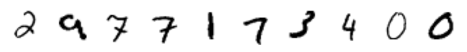
Before we continue to set up our model, we first have a look at a few randomly sampled images from our training data:

plt.figure()

images = [train_dataset[i] for i in np.random.choice(len(train_dataset), 10)]
for i, (image, _) in enumerate(images):
    plt.subplot(1, 10, i+1)
    plt.imshow(image[0], cmap='binary')
    plt.axis('off')

plt.show()

Defining the Model

After we had a look at the data, we can define our model. We use convolutional layers in the encoder and scale the hidden representation up in the end.

class Encoder(nn.Module):

    def __init__(self):
        super().__init__()
        self.conv = nn.Sequential(
            nn.Conv2d(1, 32, 3),
            nn.ReLU(),
            nn.Conv2d(32, 64, 5),
            nn.ReLU(),
            nn.MaxPool2d(2),
            nn.Conv2d(64, 64, 5),
            nn.ReLU(),
            nn.MaxPool2d(2)
        )
        self.fc_mu = nn.Linear(576, 16)
        self.fc_logvar = nn.Linear(576, 16)

    def forward(self, x):
        z = self.conv(x)
        z = z.view(z.size(0), -1)
        return self.fc_mu(z), self.fc_logvar(z)


class Decoder(nn.Module):

    def __init__(self):
        super().__init__()
        self.fc = nn.Linear(16, 2048)
        self.conv = nn.Sequential(
            nn.ReLU(),
            nn.ConvTranspose2d(128, 64, 5, stride=2),
            nn.ReLU(),
            nn.ConvTranspose2d(64, 32, 5, stride=2, padding=1),
            nn.ReLU(),
            nn.ConvTranspose2d(32, 1, 6)
        )

    def forward(self, x):
        z = self.fc(x)
        z = z.view(-1, 128, 4, 4)
        return self.conv(z)


class VAE(nn.Module):

    def __init__(self):
        super().__init__()
        self.encoder = Encoder()
        self.decoder = Decoder()

    def forward(self, x):
        mu, logvar = self.encoder(x)
        std = (0.5 * logvar).exp()
        eps = torch.randn_like(std)
        z = mu + eps * std
        return self.decoder(z), mu, logvar

Having defined the model, we can initialize it. Let’s also see how big it is:

model = VAE()

print(f'Total parameters:   {sum(p.numel() for p in model.parameters()):6,}')
print(f'Encoder parameters: {sum(p.numel() for p in model.encoder.parameters()):6,}')
print(f'Decoder parameters: {sum(p.numel() for p in model.decoder.parameters()):6,}')

Total parameters:   464,577
Encoder parameters: 172,512
Decoder parameters: 292,065

Training the Model

optimizer = optim.Adam(model.parameters())
loss = xnn.VAELoss(nn.BCEWithLogitsLoss(reduction='none'))
engine = xnn.AutoencoderEngine(model, expects_data_target=True)

history = engine.train(
    train_loader,
    val_data=val_loader,
    epochs=50,
    eval_every=5,
    optimizer=optimizer,
    loss=loss,
    callbacks=[
        xnn.BatchProgressLogger()
    ]
)

Epoch 1/50:
 [Elapsed 0:00:05 | 33.81 it/s] loss: 224.27307, val_loss: 159.77618
Epoch 2/50:
 [Elapsed 0:00:03 | 48.45 it/s] loss: 136.16475
Epoch 3/50:
 [Elapsed 0:00:03 | 47.73 it/s] loss: 118.60185
Epoch 4/50:
 [Elapsed 0:00:03 | 47.37 it/s] loss: 113.22937
Epoch 5/50:
 [Elapsed 0:00:03 | 48.84 it/s] loss: 110.84675
Epoch 6/50:
 [Elapsed 0:00:05 | 33.62 it/s] loss: 109.05308, val_loss: 108.66338
Epoch 7/50:
 [Elapsed 0:00:03 | 48.16 it/s] loss: 107.91442
Epoch 8/50:
 [Elapsed 0:00:03 | 48.23 it/s] loss: 106.88257
Epoch 9/50:
 [Elapsed 0:00:03 | 48.17 it/s] loss: 106.14308
Epoch 10/50:
 [Elapsed 0:00:04 | 46.60 it/s] loss: 105.65662
Epoch 11/50:
 [Elapsed 0:00:05 | 32.55 it/s] loss: 104.96011, val_loss: 105.40081
Epoch 12/50:
 [Elapsed 0:00:03 | 47.57 it/s] loss: 104.49724
Epoch 13/50:
 [Elapsed 0:00:03 | 48.58 it/s] loss: 104.16228
Epoch 14/50:
 [Elapsed 0:00:04 | 46.98 it/s] loss: 103.70670
Epoch 15/50:
 [Elapsed 0:00:03 | 47.52 it/s] loss: 103.35032
Epoch 16/50:
 [Elapsed 0:00:05 | 32.94 it/s] loss: 102.94538, val_loss: 104.24427
Epoch 17/50:
 [Elapsed 0:00:03 | 47.96 it/s] loss: 102.75075
Epoch 18/50:
 [Elapsed 0:00:03 | 47.43 it/s] loss: 102.43628
Epoch 19/50:
 [Elapsed 0:00:04 | 46.99 it/s] loss: 102.14312
Epoch 20/50:
 [Elapsed 0:00:03 | 48.86 it/s] loss: 102.00880
Epoch 21/50:
 [Elapsed 0:00:05 | 34.45 it/s] loss: 101.70227, val_loss: 102.42951
Epoch 22/50:
 [Elapsed 0:00:03 | 47.53 it/s] loss: 101.51430
Epoch 23/50:
 [Elapsed 0:00:03 | 47.14 it/s] loss: 101.41744
Epoch 24/50:
 [Elapsed 0:00:03 | 48.21 it/s] loss: 101.11735
Epoch 25/50:
 [Elapsed 0:00:04 | 46.84 it/s] loss: 100.98458
Epoch 26/50:
 [Elapsed 0:00:05 | 34.03 it/s] loss: 100.77367, val_loss: 101.82356
Epoch 27/50:
 [Elapsed 0:00:03 | 47.59 it/s] loss: 100.74920
Epoch 28/50:
 [Elapsed 0:00:03 | 47.90 it/s] loss: 100.51038
Epoch 29/50:
 [Elapsed 0:00:03 | 47.73 it/s] loss: 100.34299
Epoch 30/50:
 [Elapsed 0:00:03 | 47.22 it/s] loss: 100.36984
Epoch 31/50:
 [Elapsed 0:00:05 | 34.22 it/s] loss: 100.08789, val_loss: 101.58796
Epoch 32/50:
 [Elapsed 0:00:03 | 47.51 it/s] loss: 99.98875
Epoch 33/50:
 [Elapsed 0:00:03 | 47.47 it/s] loss: 99.85116
Epoch 34/50:
 [Elapsed 0:00:03 | 47.31 it/s] loss: 99.75701
Epoch 35/50:
 [Elapsed 0:00:03 | 48.25 it/s] loss: 99.61550
Epoch 36/50:
 [Elapsed 0:00:05 | 33.42 it/s] loss: 99.44988, val_loss: 100.72999
Epoch 37/50:
 [Elapsed 0:00:03 | 47.57 it/s] loss: 99.42586
Epoch 38/50:
 [Elapsed 0:00:03 | 47.50 it/s] loss: 99.36446
Epoch 39/50:
 [Elapsed 0:00:03 | 47.76 it/s] loss: 99.26171
Epoch 40/50:
 [Elapsed 0:00:03 | 48.82 it/s] loss: 99.17992
Epoch 41/50:
 [Elapsed 0:00:05 | 33.88 it/s] loss: 99.09690, val_loss: 100.31133
Epoch 42/50:
 [Elapsed 0:00:03 | 47.69 it/s] loss: 98.97497
Epoch 43/50:
 [Elapsed 0:00:03 | 49.46 it/s] loss: 98.90181
Epoch 44/50:
 [Elapsed 0:00:03 | 48.44 it/s] loss: 98.79760
Epoch 45/50:
 [Elapsed 0:00:03 | 48.53 it/s] loss: 98.63344
Epoch 46/50:
 [Elapsed 0:00:05 | 33.40 it/s] loss: 98.56735, val_loss: 100.23586
Epoch 47/50:
 [Elapsed 0:00:04 | 46.33 it/s] loss: 98.47528
Epoch 48/50:
 [Elapsed 0:00:04 | 45.59 it/s] loss: 98.47498
Epoch 49/50:
 [Elapsed 0:00:03 | 47.31 it/s] loss: 98.40941
Epoch 50/50:
 [Elapsed 0:00:05 | 33.68 it/s] loss: 98.32704, val_loss: 100.99587

Inspecting the Model

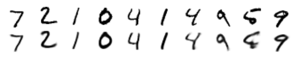
Reconstructing Images

reconstructed = engine.predict(
    test_loader,
    reconstruct=True
)

plt.figure(dpi=150)

im = next(iter(test_loader))
for i in range(10):
    plt.subplot(1, 10, i+1)
    plt.imshow(np.concatenate([
        im[0][i][0].numpy(),
        reconstructed[0][i].sigmoid().numpy().reshape(28, 28)
    ]), cmap='binary')
    plt.axis('off')

plt.show()

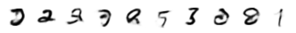
Generating Images

dim = 16
distribution = D.Normal(torch.zeros(dim), torch.ones(dim))
dist_data = xnn.NoiseDataset(distribution)

generated = engine.predict(
    dist_data.loader(batch_size=10),
    iterations=1,
    reconstruct=False
)

plt.figure()

for i in range(10):
    plt.subplot(1, 10, i+1)
    plt.imshow(generated[i].sigmoid().numpy().reshape(28, 28), cmap='binary')
    plt.axis('off')

plt.show()